Finding cars on satellite imagery – Part 3

It has been a little while since I’ve had a chance to update this blog but the stars have realigned and there should be a few more updates over the coming weeks. I really want to finish off this project but before I can make more steps forward, I have to take one step back.

Car_Clicker Updated

The method I was using for locating cars in the training data was not adequately centring on the car. Just to remind us what was happening – I had an .exe in autohotkey that loaded one of my scraped satellite images from google maps and then allowed me to click on cars to record their location. The click drew a box around the car and so I was able to verify that the car was roughly centred in the box. The downsides of this method are I didn’t have a way to remove the box if the car wasn’t centred and I was only using my eye to guess the centre position.

Now, I have recreated the autohotkey script in python using tkinter to display the image and allow me to use the mouse to locate the car. The new method allows me to click and hold on one corner of a car and then drag the mouse to the diagonally opposite corner. A circle is drawn around the centre point between where the mouse was first pressed and the current position. The circle is a good way to check that the car is centred before I release the mouse. The image below shows this step. When the mouse is released, a green box is drawn around the car so I can easily see which cars are yet to be entered into the training set. I also now have the ability to remove the last recorded location with a right-click.

car_clicker
Three cars have already been located (green squares) and one car is currently being selected (white circle). When the LMB is released, the centre location is recorded and a green box drawn.

I am hoping that training the convnet on more accurately centred cars will return a smaller probability blob centred on the car in the final classification phase. More results to come soon from this.

Archiving and backing up to Amazon S3

The second update I have made to the project is to code up a couple of classes – Archive and S3Bucket. These allow me to keep a list of all the files I have written when a script runs and then archive them into a gzipped tarball. The archive can then be either written to disk or uploaded to an S3 bucket on AWS.

The reason I am doing this is to have a more robust backup of the work I am doing. All of the scripts are synced to GitHub but none of the script outputs were backed up anywhere. I had a minor scare when I formatted my computer as I thought I had lost everything! Luckily I had backed it up to another machine but there was definitely some panic before I remembered that!

To communicate with AWS, I am using the Boto3 python library (link). It makes it relatively straightforward to implement all of the functions available in the AWS SDK. I think it might be worthwhile to list the steps to implement something like this from a data scientist’s perspective (i.e. not a software engineer so apologies if this is obvious).

  1. Log into the AWS console.
  2. Create an IAM user and select a Group that does what you want. I limited mine to S3FullAccess and will increase the security in the Bucket itself.
  3. Create an S3 Bucket that Boto3 will send files into.
  4. Set up the Bucket Policy to deny DeleteObject and DeleteObjectVersion on the items in the bucket (resource/*).
  5. Also deny DeleteBucket and DeleteBucketPolicy on the Bucket resource (this way if your IAM user details are compromised the archive data cannot be deleted).
  6. Configure Boto3 to use the IAM user credentials.

My archive class automatically provides a name that consists of the script that was called to produce it and then it is made unique by appending the date and time to the end. I have been including these two classes in all of my car counting project scripts to automatically archive any created files.

Finding cars on satellite imagery – Part 2

Following on from my previous post, I have some results and conclusions on this project.

I trained the convnet for 100 epochs in the previous post and for this work I will use the 70th epoch. It has a good precision and recall of 0.952 and 0.922 respectively. Combined, the F1 score is 0.937. The epochs around this seem to oscillate a little bit between precision and recall and this particular version seems to have a good trade-off between the two.

figure_070

So I loaded up this convnet and rasterised 5 test images into 40×40 pixel images. The probability map is then plotted on top of the image with the centre of the 40×40 image displaying the value. Because of this there is a 20 pixel border where no predictions are made so any cars in this region probably won’t be identified. The results are quite encouraging with most cars being detected. These images were chosen by me and a I tried to gather some images that are similar to the training data and some that are different. None of these images overlap with the training data set and they are completely unseen by the convnet until now.

In this image, there are some false negatives of cars in the shade. False positives include the area around the tree, the roof-line as well as some of the area near the rail track. Overall, the convnet does well with this image (just my opinion – I will formalise the efficacy in a future post).

This was another image that is similar to the training data although the angle of the street is different. It misses (false negatives) a few of the dark coloured cars on the street and the parking lot and incorrectly identifies some of the roof-lines as high probability cars. Again, the convnet performs admirably but it definitely needs improvement.

I chose this image because of the different angles of the aligned cars and the large grassed area is something that wasn’t included in the training dataset. All of the cars have been found but the two sheds in the centre of the image have been mislabelled. There are also some trees and roof lines that have been identified as cars.

The air-conditioning units and some of the pool equipment makes up the false positives in this image. All of the cars are found so this image has a lot more false positives than false negatives.

The darker tones and trees in this image are very different to anything the convnet saw in training. Consequently it doesn’t do very well when it comes to false positives as it finds a lot of them. It does identify all of the cars as far as I can tell so again, false positives far outweigh the false negatives.

This last image is of the ocean and there was no images at all like this in the training dataset. There are a lot of false positives in this image mainly due to the reflections from the sun on the waves. It would definitely be worthwhile to include some images like this in the training data on future training runs.

Overall the convnet does pretty well with these test images. There are something like 300,000 raster images per image so with a precision and recall of 95% you would expect 15,000 false positives and negatives. It would seem that this is roughly what we are seeing in the later images but it is performing better than this in the first few images. The best thing to do from here would be to include more training images from different locations. I can also vary the probability threshold a little to make some trade-offs between false positives and negatives. Some more analysis to come in a future post.

Finding cars on satellite imagery

For the last week or so, I’ve been working on a little project that will be able to find cars from a satellite image. I will be using images from Google Maps centred around Brisbane and hope to increase the labelled dataset to other cities in the near future. This project was coded in python 3.5 using Keras to access TensorFlow and can be found on my github page github.com/TheZepto/Car_Counter.

Scraping and labelling

I’m approaching this project from scratch – so no Googling “satellite image labelled dataset”. It wasn’t too difficult to get the Google Static Maps API working to download a chunk of Brisbane satellite images at a resolution that makes cars obvious. I chose to use a 10×10 grid of images that all have a size of 640×640 px. A few example images are below. I tried to find an area of the city that included residential as well as built up areas with different types of carparks included. In the script, I ignore the bottom 20 px so as to not include the text.

Now that I have all of these images, the next step was to manually find the location of the cars. I used a GUI that a friend of mine built using AutoHotKey that loads an image, records the location of a click in a text file and then draws a 40×40 box around the location of the click. The text files are in the format of row, column of the press. In this way I end up with text files for each image that contains the centre location of each car. Using this utility, I was able to process 100 images in about 40 minutes and ended up with 1700+ images of cars. Below is a screen capture of the car_clicker.exe utility.

car_clicker

Now that I have all of these images and corresponding txt files containing the centre locations of the cars, I wrote a python script that loads the images into a 640x640x3 numpy array and the text file into a [n_cars]x2 numpy array. As I mentioned above, the bottom 20 rows of the numpy array are discarded to avoid any text making it into the image set. I use a class to hold the image and there is a method that will remove a specified number of rows from the image array.

The image class contains another method that will return a cropped square image based on a centre position and a size. I will refer to this as a region-of-interest or ROI. The first step in creating the ROI is to check that it is valid, i.e. that it exists wholly inside of the main image. If it is a valid selection then the cropped image is returned and stored and saved into an array of size [n_cars]x40x40x3. For this project, the size of my cropped images is 40×40 as this seems to be an appropriate size to just include the car and not much else. For this project to be successful, I need to be able to identify images with a car in the centre not just whether there is a car somewhere in the image. A 40×40 image is just large enough to ensure this. Below are some images of the cars that were taken out of the above image.

02_cars

In order to generate the “not-cars” labelled data, I use a rolling window with the same size of 40×40 but with a stride of 50 so as to not overlap the data too much. In order to not have any cars in this data, each ROI centre is checked to make sure it is at least a set distance from the centre of the known car locations. I used a value of 15 for the distance and this is just using a standard vector distance as opposed to number of pixels – it is a little easier to check this way. 15 is a good value to use because it will include some images that have a car that is not centred in the image. Only images with cars centred in the image should be labelled as cars so this will help the training of the machine learning algorithm later. I have taken some of the “not-cars” images from the same image as before, below.

02_notcars

Both of the labelled data arrays are then saved as numpy arrays so they can be combined later. I chose this methodology as opposed to just processing all of the images at once in the script so that it can be scaled up and down in the future. The biggest limiting factor is that I was only able to scrape 640×640 px images from Google Maps which is why I have 100 images in a 10×10 grid instead of just one 6400x6400px image. The piece-wise nature of the processing also allows for me to reprocess files if they contain errors or I accidentally click on something that isn’t a car – a mistake that happens quite a lot after 80 images!

Combining the data into training and testing sets

At this stage, I have 100 saved arrays of X0 (the negative “not-cars” images) and X1 (the positive “cars” images). Both of these need to be combined, shuffled and split into a training and testing dataset. I also need to create the corresponding Y array filled with 0 and 1 based on if the corresponding image is a car or not. Care has to be taken to not mix the indices around otherwise images will end up being mislabelled.

After combining all the arrays and splitting it, I am left with:
Training data: 12544 total images with 1382 images of cars
Testing data: 3136 total images with 346 images of cars

The number of cars in the training data is a little low and at some point I will increase it by using some image transformations. By rotating, shifting and flipping the data in a random fashion, the number of car images could be increased by a factor of 10. It should be noted that rotation is probably the most important transformation I could perform as most of the images I have are all similarly aligned. As cars are usually on roads or parked besides roads, the road axis determines the orientation of most of the cars. I have attempted to negate this by introducing a rotation transformation as a data augmentation before the convnet is trained – more details of this will be given in the next section.

The script saves the data as 4 arrays: X_test, X_train, Y_test and Y_train. Most networks take these inputs and it is exactly what is needed for Keras. In the next section I will look at training a simplistic convolutional neural network on the data I have.

Training a simple convolutional neural network

The network architecture is the same as I used from my last blog post (here). It had okay classification results with 10 classes and I aim to get >90% accuracy at classifying cars with it. This project is more of a proof of concept so no doubt there will be a lot of room for optimisation of this step even once I am done. Here are the layers of the convnet: convolutions consist of 3×3 filters, activations are rectified linear with softmax at the output, pooling size is 2×2, and dropouts are 25% to prevent overfitting.

model

The training that I will do will use realtime data augmentation to alter the images randomly within a range of given parameters. This will ensure that the network will never really see the exact same image twice and should improve its ability to classify cars in images outside of the ones given. I will use a rotation of 20 degrees, and horizontal and vertical flip. Using the horizontal and vertical shift wouldn’t be a good idea for this network as I want to classify images that are centred on a car. There is already some variability in the centring that was introduced by me approximating the location when labelling the data, so I don’t want to increase this any further. I am using Keras’ image pre-processing for this step.

I have used the same code as that last project so the confusion matrix is saved for each training epoch. It is a little updated so that I am now using a callback function in Keras, rather than running the fit method in a for loop. The model is also being saved after each epoch so I should be able to pick the optimally trained model and use it to identify cars in images.

giphy (3)

The training seems to be optimal around the 50th epoch and then it oscillates a bit between precision and recall for ever other iteration. This seems to indicate that the learning rate needs to be reduced a little after epoch 50. However, for this project I find that epoch 70 has a very good precision and recall of 0.95224 and 0.92197 for a combined F1 score of 0.93688. This meets the criteria that I set for an accuracy at classifying of >90% so I will declare this a success and carry on!

To be continued…

Investigating training progress of ConvNets [Keras]

I’ve recently been implementing some convolutional neural networks and have been thinking about good ways to check how the network is learning. The most obvious way is to monitor the accuracy and logloss after each training epoch of both the training and validation data. Another way I want to look at the training progress is to generate a confusion matrix after each epoch to give some insight into what classifications are having trouble being trained.

Network setup

I’m running Keras on Python 3.5 and mainly working with the included CIFAR-10 example. The backend is TensorFlow with GPU acceleration on my GTX 970. It was definitely worth the extra bit of hassle to get GPU acceleration working because the training was taking 10x longer on my CPU (i5 4570), 200 seconds per epoch compared to 18 seconds! The network that I will use has a total of 1,250,858 trainable parameters.

model

The network architecture is displayed above. It is a sequentially layered network that has a reported logloss of 0.65 after 25 epochs and then 0.55 after another 25 epochs. I was unable to recreate these results after running 3 times. However, I will keep trying and report more on the reliability later. I’m also toying with the idea of including some Inception modules and residual learning layers to improve the architecture and training times. At that point though it is probably just quicker to start using inception-v4 or inception-resnet directly. I’ll follow this up in a later blog post, for now I am just going to explore the above network. The code that I am using can be found on my Github (link).

The Keras example that I am basing this blog post on also uses real-time data augmentation on the training data. The augments that are being used are a horizontal and vertical shift that is random for each epoch with a range of 10% of the total width. There is also a random horizontal flip that will reverse the image. By including these pre-processing steps, the versatility of the algorithm can be improved.

Results

giphy
Run 1
giphy (1)
Run 2
giphy (2)
Run 3

I’ve assembled the confusion matrices of the first 3 runs of the training into gifs. I trained over 100 epochs and give 1-10 and then every 10th. The first 10 epochs have the largest training difference and the gif really makes it easy to see the improvement. Essentially this image dataset is made up of vehicles and animals and it is interesting to note that the ConvNet can distinguish between these two classifications quite well from the start. There is some difficulty in differentiating between cats and dogs and automobiles and trucks, for example. Most of the vehicles have common features between them and the same goes for the animals. It would be a big red-flag if the algorithm was unable to distinguish between an animal and a vehicle!

This algorithm was claimed to have a tested LogLoss of 0.55 after 50 epochs but I don’t observe this. The best that I was able to achieve was 0.6109 after 80 epochs as observed on run 3.

I hope to return to this network in the near future and try to work out why I am unable to observe similar performance. I am also planning to look at optimising the computation time by varying the batch size used per epoch (it was 32 in this work). It would also be great to improve upon the results by including some different layers such as Inception and residual learning. So much I want to look at, but it takes 30 minutes to run 100 epochs which is slowing down my progress!

Finalising the analysis of predicting leaving employees [HR dataset part 3]

In part 2, I looked at finding the optimal hyperparameters for the 3 most accurate learning algorithms and see which of the methods best suited the HR dataset from kaggle.com. The clear winner in part 2 (and also part 1) is the random forest classifier. Now that it is operating optimally, it is time to evaluate the final performance to see how well it can predict employees leaving and staying.

All of the testing done below is performed on a 20% split (or 3000 total) of the dataset that was put aside specifically for this final evaluation. None of the data used in the analysis has been used for cross-validation or training. In this way, I don’t have to worry that the algorithm is only good at operating on the training and cross-validation datasets.

The first visualisation to produce is a confusion matrix. This shows the difference between the predicted and true outcome labels. For the random forest classifier this matrix is given below.

Conf_Matrix

We can clearly see from the matrix a few important statistics. The diagonal SW and NE corners were predicted incorrectly while the NW and SE corners were correct. A total of 30 cases were incorrectly predicted which represents 1% of the total data so it is clear that the random forest classifier is doing an excellent job. From the matrix the precision and recall scores can also be calculated for predicting the employees who leave. The precision is 0.989 and the recall is 0.969 to give a combined F1 score of 0.979.

At this point it is important to consider what the ultimate goal of this project: can some stayers be misidentified as leavers in order to ensure more leavers are correctly identified? At the moment, the classifier makes a decision based on a continuous variable output on the final layer. This value ranges from 0 to 1 with predictions >0.5 being labelled as leaving, otherwise they are identified as staying. A good visualisation in order to illustrate this concept a little better is to generate an ROC curve (Receiver Operating Characteristic).

An ROC curve essentially varies the prediction threshold over a range from 0 to 1. If the prediction threshold is set to 0 then everything will be identified as having a label of 1 and vice-versa. The true positive (TPR) and false positive rate (FPR) at each threshold is then plotted to form the curve. Below is the ROC curve for the random forest classifier.

ROC


The curve shows the effect of improving the odds of identifying all leavers by increasing the chances of misidentifying staying employees as leavers. With the default threshold of 0.5 there was a recall (or TPR) of 0.969. Decreasing this threshold we can see the TPR increases to greater that 0.98 but the FPR increases to 0.025. Therefore  we can correctly identify an extra 1% of the number of leavers by misidentifying 2.5% of stayers as leavers. I would suggest that this is a more favourable outcome for the project. Ultimately a decision like this would come down to the financials: how much does it cost to incentivize employees to stay versus the cost of recruiting new employees. The ROC curve is the ideal way to make this determination.

To wrap up this analysis, the random forest classifier is superior to all other methods that I tried in these series of posts. By optimising the hyperparameters with a grid-search, the overall effectiveness of the algorithm was increased by 1-2% over the default settings used in scikit-learn. The final decision as to what prediction threshold should be used is best decided by the ROC curve and I would suggest decreasing this threshold to increase the detection rate of employees leaving while misidentifying some stayers.

All of the code used in this analysis can be found on my github, as a publicly available repo.

Visualising Queensland road crash data with Tableau

I have a database of road crash data for Queensland from 2001 to 2010 that is perfect for doing some data visualisation on. Travelling on the roads is a risk that we encounter everyday but are the roads getting safer? Are there safer times of the day to travel? Let’s have a look at some of the data to try to answer these questions and see if any trends become apparent.

For this I will be using Tableau. It is a great application for easily throwing together visualisations from raw data formats. I prefer to use Tableau when first exploring data as it is more powerful than Excel while not requiring a lot of the pre-processing steps when using python+matplotlib or R+ggplot2. The graphs that it produces look great from the start and saves a lot of beautification time in Illustrator. Most of the other graphs on this blog are straight out of matplotlib and they are nowhere near as pretty as these.

Casualties & fatalities geo-distribution

I was able to generate some rectangular bins in latitude and longitude to group the data into regions. Most of the regions are centred on major highways in Queensland as the position of the marker is placed at the average lat. and long. for the bin. Rectangular bins can look odd when placed on a map if careful consideration isn’t taken to operate in polar coordinates.

Looking at the graph below, we can clearly see that most of the casualties in Queensland happen in the south-east region and then along the east coast. The total fatalities also are reasonably uniformly distributed around population centres. There are no real surprises in this data set, for example there are no regions that show disproportionate numbers of fatalities. This figure also shows the data for two year ranges.

Crash Data Geoprojection


This figure also shows the data for two year ranges: 2001 to 2005 and 2006 to 2010. Very little changed in terms of absolute number of casualties and fatalities and the spread of the data over the map also looks similar. This would imply that the number of accidents in Queensland was more or less uniform in these two year ranges. Instead of plotting the absolute number of casualties and fatalities, the relative number of fatalities per reported casuality can also be looked at. This way it is more apparent if there are regions that have disproportionately high numbers of fatalities.

Crash Data Geoprojection Fatalities


In this figure, the small dark red dots that appear in the west of the state are regions were there were few accidents but the accidents that did occur resulted in a fatality. It appears that little changed from 2001-2005 to 2006-2010. The other interesting thing from this figure is how the Brisbane region recorded the most casualties but actually had one of the lowest number of resulting fatalities.

Injury types

Now that we have looked at the breakdown of accidents in different regions of Queensland, we can look at the types of injuries and treatments required. If the state is now considered as a whole, the breakdown of the type of casualties can be graphed over the years from 2001 to 2010.

Treatments

It is good to see the fatality count trending downwards over the years. Interestingly, the number of people hospitalised after a crash is increasing over time. The number of people to receive some medical treatment is roughly constant with no obvious trend either up or down over the timeframe looked at. Minor injuries had a large peak in 2007 and if we ignore this outlier, the general trend is decreasing. A decrease in minor injuries is most likely due to increasing safety standards in cars. From this data, it would appear that the increase in hospitalisation and more safe cars are reducing the number of fatalities in Queensland.

Type of crash

The final thing to look at is the type of accident that occurs on the roads. For this I will use the top 10 crash natures: angle collisions, rear-end collisions, hit objects, overturned vehicles, sideswipe collisions, hit parked vehicles, hit pedestrian, fall from vehicle, head-on collision, and hit animal.Accident causes

If we look at the type of accident happening during different times of the day, we can see that during daylight hours is when most crashes occur. The thing that jumps out at is the large increase at 3pm – when school generally finishes. At 8am and 3pm, we observe large increases in the number of rear-end crashes and hit pedestrians. This graph really illustrates why school zones were introduced as an attempt to decrease the number of accidents around these times. It is interesting to see that angle and rear-end collisions dramatically decrease during night and the number of hit animal accidents increases around sunrise and sunset.

The nature of crashes over the period of 2001-2010 do not seem to change appreciably with the total number of accidents reported not varying by any more than 5%. Of course this doesn’t take into account that the population of Queensland increased from 3.8 million to 4.3 million during this time. Thus we can conclude that there is actually a 10-15% decrease in the number of accidents per capita.

Final thought

Overall it would appear that the number and distribution of road crashes in Queensland was stable over the years 2001-2010. Most of the crashes occur in the south-east region, followed by rest of the east coast, and not many crashes in the west. This aligns with the population distribution of Queensland. There are trends towards increased hospitalisation, decreased minor injuries, and decreased fatalities. As the number of people requiring medical treatment has remained steady, it is reasonable to conclude that serious accidents are becoming more rare most likely due to increased car and road safety. The majority of road accidents happen during daylight hours with increased occurrences during the morning and afternoon rush hours (8-9am and 3-7pm).

The number of accidents have remained constant from 2001-2010 but due to the population increase, the per capita statistic has improved. To make more concrete conclusions as to whether Queensland roads are getting safer from this data I would also like to include population and the number of registered vehicles in the analysis. This would give a more complete picture in terms of per capita and per vehicle accidents. Unfortunately I haven’t been able to find all of this data, but will post an updated version of this visualisation if I find it in the future.

A “sharebrained” idea

In this blog post, I want to chronicle my first naive efforts at implementing deep learning. The project never worked but I learnt quite a lot about the process along the way and I think it might be useful for people who are starting out.

After completing the machine learning course of Stanford University I was keen to try my new skill set on some problems. “How about I try to predict share price movement?”, I thought. It seems like a complicated problem but there are numerous examples of it working well enough in the literature and maybe I would be able to earn a few bucks on the side. I chose a neural network architecture for no reason other than they interest me the most. I thought that a regression problem might be too difficult to predict the future value of shares so I decided to make it into a classification problem that would answer the question: will share price increase tomorrow? The project was codenamed ShareBrain.

Scraping the data and preparing the training examples

I used python as the scripting language and found a yahoo-finance package that would download historical data for a given share. The package returned the data in a dictionary list. The below code is my implementation of scraping the data and then saving it in a file locally. If this file already existed then it would be loaded to save downloading it all again.

import sys
import numpy as np
from yahoo_finance import Share #The yahoo-finance package is used to gather the share data

# Srape historical share data
# Inputs:
# - share_name as given by yahoo finance
# - start_date and end_date as yyyy-mm-dd for the range of historical data to find
# - use_existing_data will try and use pre-fetched and stored data if True
# Returns:
# - historical_data in list form ordered oldest to newest
def get_share_data(
	share_name='ANZ.AX',
	start_date='2005-01-01',
	end_date='2016-01-01',
	use_existing_data=True):

	share_filename = 'Data/' + share_name + '_' + start_date + '_' + end_date +'.npy'

	if use_existing_data:
		try:
			historical_data = np.load(share_filename).tolist()
			print("Data successfully loaded from locally stored file")
		except:
			#Scrape the data for the given settings and exit if there is an error
			print("Attempting to scrape data for", share_name)
			try:
				historical_data = Share(share_name).get_historical(start_date, end_date)
				np.save(share_filename, historical_data)
			except:
				print("Error in scraping share data. Share name is probably incorrect or Yahoo Finance is down.")
				quit()
			print("Scrape succesful")
	else:
		print("Attempting to scrape data for", share_name)
		try:
			historical_data = Share(share_name).get_historical(start_date, end_date)
			np.save(share_filename, historical_data)
		except:
			print("Error in scraping share data. Share name is probably incorrect or Yahoo Finance is down.")
			quit()
		print("Scrape succesful")

	# Reverse the order of the historical data so the list starts at start_date
	historical_data.reverse()

	return(historical_data)

The values that I wanted from the historical data were the opening, closing, high and low prices, as well as the volume of shares traded. Now to form the training data for the neural network I grouped together these data points for a number of days. The default value was for 30 days worth of data to be concatenated in an overlapped fashion (i.e. day 1 to day 30, then day 2 to day 31, then day 3 to day 32, etc.) The classifier was then set up to give a label of 1 if the next day’s closing share price was greater than the closing share price of the last day in the training input, otherwise the example was labelled as 0. The below code performs these steps and returns a numpy array with training examples set up in each row.

# Process the historical share data with boolean training target
# Inputs
# - historical_data as returned from get_share_data
# - days_of_data is the number of consecutive days to be converted into inputs
# Returns
# - training_input array with the share's volume, high, low, open, and close price for
#   the number of days specified in days_of_data between the start_date and end_date.
# - training_target array consist of a boolean value indicating if the closing price
#   tomorrow is greater than the closing price today.
def proc_share_bool_target(
	historical_data,
	days_of_data=30):

	# Process the returned data into 3 lists of: open_price, close_price, and volume
	try:
		open_price = [float(historical_data[i]['Open']) for i in range(0,len(historical_data)) ]
		close_price = [float(historical_data[i]['Close']) for i in range(0,len(historical_data)) ]
		volume = [float(historical_data[i]['Volume']) for i in range(0,len(historical_data)) ]
		high_price = [float(historical_data[i]['High']) for i in range(0,len(historical_data)) ]
		low_price = [float(historical_data[i]['Low']) for i in range(0,len(historical_data)) ]

	except ValueError:
		print("Error in processing share data.")
		quit()

	# Take the historical data and form a training set for the neural net.
	# Each training example is built from a range of days and contains:
	# the open and close share price on each day in the range.
	# The output is boolean indicating if the close price tomorrow is greater than today.

	training_input = np.array([])
	training_target = np.array([])

	training_example_number = len(open_price) - days_of_data

	for i in range(0, training_example_number):
		training_input = np.append(training_input, volume[i:i+days_of_data])
		training_input = np.append(training_input, high_price[i:i+days_of_data])
		training_input = np.append(training_input, low_price[i:i+days_of_data])
		training_input = np.append(training_input, open_price[i:i+days_of_data])
		training_input = np.append(training_input, close_price[i:i+days_of_data])
		training_target = np.append(training_target, close_price[i+days_of_data] > close_price[i+days_of_data-1] )

	# The above for loop makes 1-dim arrays with the values in them. Need to use reshape
	# on training input to make it 2-dim. Number of columns is 3*days_of_data to account for
	# open price, close price and volume. The -1 in reshape will be filled
	# automatically and (days_of_data +1) is the number of columns for each input. Likewise
	# for the target array.

	training_input = np.reshape(training_input, (-1, 5*days_of_data))
	training_target = np.reshape(training_target, (-1,))

	return (training_input, training_target)

Implementing the neural network

I used scikit-learn to perform the neural network training and my plan was to test different levels of complexity by varying the number of hidden layers and neurons. The standardscaler provided in this library also was useful in normalising the columns of the training array to have a range from -1 to +1. The training step was placed in a loop that would retrain the algorithm until a certain accuracy was attained (it is set to 10% below for reasons that will become clear soon).

# Common libraries
import sys
import numpy as np
import matplotlib.pyplot as plt

from sklearn.model_selection import train_test_split
from sklearn.preprocessing import StandardScaler
from sklearn.neural_network import MLPClassifier

# My libraries
import sharescraper

# Boolean prediction of whether the close_price tomorrow will be greater than today.

# Get training input and targets from sharescraper
historical_data = sharescraper.get_share_data(
	share_name='ANZ.AX',
	start_date='1920-01-01',
	end_date='2016-01-01',
	use_existing_data=True)

(price_input, boolean_target) = sharescraper.proc_share_bool_target(
	historical_data,
	days_of_data=10)

# Separate data into training set and test set
random_number = 0
test_split = 0.3
X_train, X_test, y_train, y_test = train_test_split(
	price_input, boolean_target, test_size=test_split, random_state=random_number)

# Feature scale the training data and apply the scaling to the training and test datasets.
scaler = StandardScaler()
scaler.fit(X_train)
X_train = scaler.transform(X_train)
X_test = scaler.transform(X_test)

# Set up the MLPClassifier
clf = MLPClassifier(
	activation = 'tanh',
	learning_rate = 'adaptive',
	solver ='adam',
	hidden_layer_sizes=(10),
	alpha = 0.01,
	max_iter = 10000,
	tol = 1E-8,
	warm_start = False,
	verbose = True )

# Train the network on the dataset until the test_accuracy raches a threshold
accuracy_check = True
while accuracy_check:
	# Train the neural network on the dataset
	clf.fit(X_train, y_train)

	# Use the cross validation set to calculate the accuracy of the network
	test_accuracy = clf.score(X_test, y_test)
	train_accuracy = clf.score(X_train, y_train)
	print("The network fitted the test data {:.3f}% and the training data {:.3f}%."
		.format(test_accuracy*100, train_accuracy*100))
	accuracy_check = test_accuracy < 0.1

The mistake

When I first ran my training code I was pleasantly surprised to see that there was an accuracy of just of 60%. “Huh, that seemed to work,” I naively thought. Dollar signs began spinning in my mind as even a slight advantage over chance (accuracy of 50%) on the stock market can snowball into large gains if properly managed. There were a few minor errors here and there which I fixed up quickly – mainly to do with some data missing from the training array as I hadn’t implemented the date range correctly.

After fixing up these small errors and thoroughly debugging the code (or so I thought), I retrained the network and this time had an accuracy of over 80%, 80%! “Wow, these neural networks really work great and I haven’t even had to do very much.” “Why isn’t everyone using this method as it is proving super effective?” I thought to myself. I was expecting a small increase over chance, not something as high as 80%! With the little effort I had put into optimising the algorithm’s hyperparameters, this seemed remarkable. Too remarkable.

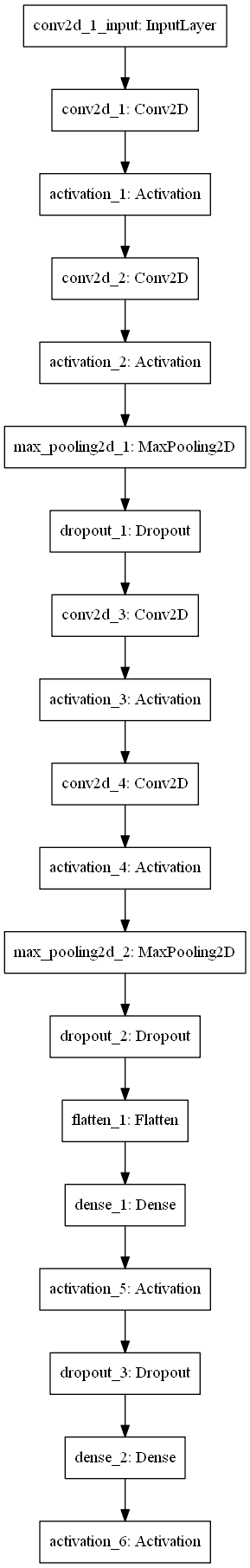
I started to toy with the hidden layers and number of neurons. The initial implementation had something like 3 layers with 100 neurons in each. So I cut that down to 2 layers with only 10 neurons in each and retrained the data. 80% accuracy. Removing more neurons and layers down to 1 layer with 5 neurons. 80% accuracy. 1 layer with 1 neuron. 80% accuracy. “Uh oh, this doesn’t seem right at all.” Could it be that the intricacies of the share market could be predicted by something simpler than a fruit fly? It certainly didn’t seem so.

This lead me on a big debugging round. What could possibly be causing my incredibly high training accuracy? It wasn’t overfitting or anything to do with regularisation. In fact changing this parameter and many others had barely any effect on the accuracy. It seemed that 80% was always attainable. I then shifted my focus to the data scraping and the mistake revealed itself. I had assumed that the data was ordered from oldest to newest in the returned dictionary list but it was actually the opposite.

Being outsmarted by a neural network

So the historical data was backwards when being used in my training set. But how would that impact the training accuracy? I first thought that it would still be the same problem just a little bit backwards with the network predicting what happened before the training data as opposed to afterwards. Surely this couldn’t be responsible. However on further inspection it makes perfect sense.

I am using the opening (O) and closing (C) price for each day and the classification is based on whether the closing price for the next day outside of the range is higher or lower than the closing price of the last day in the range. What this looks like is below.

<---------------Days in training data range---------------> <-Future
O  C  |  O  C  |  O  C  |  ...  |  O  C  |  O  C  |  O  C  |  O  C  
                                                        ^Compares^

However, this is not what I was doing as I had the dates backwards. Below is more representative of the training data and comparison that I was making.

Past-> <---------------Days in training data range--------------->
O  C  |  O  C  |  O  C  |  O  C  |  ...  |  O  C  |  O  C  |  O  C 
   ^Compares^

This is where the problem lies. In the training data the closing share price and the opening share price of the next day are the same 60% of the time. This is due to the valuation not changing when the stock market is closed from one day to the next. So all the neural network had to do was compare the opening and closing price for the one day in the range and it would be able to correctly predict the movement of the share price. The remaining 40% of the data is just being guessed with an accuracy of 50% so this adds another 20% to the accuracy which gives an overall accuracy of 80%. Mystery solved.

Moving forward

After this major problem had been solved, the accuracy of the classifier algorithm dropped back down to a more sensical 50%. I wasn’t really able to increase this any further by changing the architecture of the hidden layers and neurons. I considered adding some more contextual information in the form of scraping news websites and twitter feeds to capture community sentiment but my passion for the project had steadily declined. This was my first project and I wanted to do something that had more than a fighting chance of working. Maybe I will return to it one day and post any updates on this blog. At least I learnt a lot in how to tell if neural networks are operating correctly or whether they are just smarter than the user programming them!

The code for this project is available on my github.

Choosing optimal hyperparameters [HR dataset part 2]

This post is continuing the analysis of the HR dataset from kaggle.com. In my last blog post, I looked at a broad range of learning algorithms from scikit-learn to see what fit the dataset best. In doing this I only used the default settings for each of the algorithms (except the neural networks where I defined the hidden layers). Now I will investigate the top 3 algorithms further by tuning the hyperparameters away from the default settings. I hope to find out which algorithm will outperform the others in terms of F1 score and training time.

Methodology

The way in which I will optimise the various algorithm’s hyperparamters is to use scikit-learn’s inbuilt grid search. This allows me to enter in the parameters I would like to check over and then it will train the algorithm using all of the possible combinations. Each hyperparameter grid search is performed 5 times using a stratified K-fold cross validation set so some simple statistics can be taken to test the reliability and robustness.

def optimise_classifier_f1(clf, parameter_grid, arrInput, arrTarget):
    # Generate cross validation set
    cv_splits = StratifiedKFold(n_splits=5, shuffle=True)

    # Perform grid search over paramter grid
    grid_search = GridSearchCV(
        estimator=clf,
        param_grid=parameter_grid,
        cv=cv_splits,
        scoring='f1'
        )
    grid_search.fit(arrInput, arrTarget)

    # Performance metrics from grid search
    fit_time = grid_search.cv_results_['mean_fit_time']
    fit_time_err = grid_search.cv_results_['std_fit_time']
    test_score = grid_search.cv_results_['mean_test_score']
    test_score_err = grid_search.cv_results_['std_test_score']
    rank_test_score = grid_search.cv_results_['rank_test_score']
    params = grid_search.cv_results_['params']

    # Print each point's rank and parameters
    print()
    print("Rank and parameters for: {}".format(type(clf).__name__))
    for i,j in zip(rank_test_score,params):
        print("Rank {0:2d}  Parameters {1:}".format(i,j))

    # Plot the performance graph with each point's rank
    fig, ax = plt.subplots(1,1)
    ax.errorbar(fit_time, test_score, fit_time_err, test_score_err, 'b.')
    ax.set_xlabel('Training time (s)')
    ax.set_ylabel('F1 Score')
    ax.set_title('Evaluating {} Performance'.format(type(clf).__name__))
    for x,y,rank in zip(fit_time, test_score, rank_test_score):
        ax.annotate(rank, xy=(x,y), textcoords='data')
    plt.show()

To visualise the performance of each classifier in the hyperparamter grid search, I have chosen to plot the F1 score versus the training time. F1 score is a good indicator of combined precision/recall score and the training time looks at the complexity of the model as a more complex algorithm will take longer to train. In this manner I can also compare the training time of different algorithms. Errorbars are plotted on both axes as that is a good way to distinguish if an algorithm can be reliably trained with the hyperparameters. The plot also contains the rank that each data point came in the overall grid search. Python prints out the rank and parameters of each datapoint to the terminal so I can see what was used.

Evaluating the gradient boosting algorithm

From the initial analysis of the gradient boosting algorithm, the default settings from scikit-learn gave a F1 score of 0.94. The two hyperparameters that I will concentrate my efforts on are the number of estimators and the maximum numbers of features.

# Optimise the gradient boosting classifier
clf = GradientBoostingClassifier()
parameter_grid = {
    'n_estimators':[10, 20, 40, 80, 120, 160],
    'max_features':[i for i in range(1,10)]
}
hr.optimise_classifier_f1(clf, parameter_grid, ScaledTrainInput, TrainTarget)

GB_F1

GB_F1_zoomed

The above two figures are the results for the hyperparameter grid search, with the second figure just being a zoomed in version of the top figure. From these, it is apparent that the F1 score of 0.94 that was given with the default settings can’t really be improved on by a lot as the best performance is just above 0.95. The highest ranking F1 score (denoted by rank 1) was trained using hyperparameters of max_features=6 and n_indicators=160. I would suggest that the optimal hyperparameters for this algorithm is located at rank 20 with max_features=3 and n_indicators=80. The rank 20 datapoint has a small F1 errorbar which implies that it was reliably trained on each cross validation set. The training time errorbar is similar to all other datapoints around it, suggesting that gradient boosting isn’t having difficulty finding a solution. By chosing the rank 20 hyperparameters over the rank 1, the training time is reduced by a factor of 2.5 while the F1 score only decreases by less than 5%. In fact the errorbars of rank 1 and rank 20 overlap which implies that sometimes both algorithms train to the same F1 score.

Evaluating the 2-layered neural network

In the initial analysis of a 2-layered neural network on the dataset I used 100 and 50 neurons in each hidden layer. This gave an F1 score of 0.94, similar in performance to the gradient boosting algorithm. For the neural network I will concentrate on the regularisation parameter, alpha, and the number of neurons in each hidden layer.

# Optimise the 2-layer neural network
clf = MLPClassifier()
parameter_grid = {
    'hidden_layer_sizes':[(i,j) for i in [5,50,500] for j in [5,50,500]],
    'alpha':[0.0001, 1, 10, 1000]
}
hr.optimise_classifier_f1(clf, parameter_grid, ScaledTrainInput, TrainTarget)

NN_F1_all
NN_F1_zoomed

The results from the hyperparameter grid search on the 2-layer neural network is quite surprising in that the errorbars for the F1 score are all very large. The large error in these ponts indicates that the algorithm couldn’t be trained reliably. For each of the 5 cross validation sets there was a large range of F1 scores attained. It should also be noted that the training times are much larger than those for the gradient boosting algorithm. The 2-layered neural network algorithm can be ruled out for further investigation as it gives much worse performance. This also demonstrates why this type of analysis is important as the first impression given by the default settings of this algorithm had a performance that was in the top 3 of all tested.

Evaluating the random forest algorithm

The final algorithm to evaluate and find the optimal hyperparameters for is the random forest. This algorithm had the highest performance of all those initially evaluated with a F1 score of 0.97. The hyperparameters worth investigating are the number of estimators and the maximum number of features that the algorithm can utilise.

# Optimise the random forest classifier
clf = RandomForestClassifier()
parameter_grid = {
    'n_estimators':[i for i in range(1,20,2)],
    'max_features':[2,4,6]
}
hr.optimise_classifier_f1(clf, parameter_grid, ScaledTrainInput, TrainTarget)

RF_F1

The performance curve for this classifier algorithm cements its position as being superior to the others. All but 1 datapoint have a higher F1 score than the highest datapoint in the gradient boosting algorithm. The errorbars are also quite stable between datapoints to indicate that this algorithm can be reliably trained on the dataset each and every time. The rank 1 datapoint used n_estimators=17 and max_features=4. I would choose the rank 4 datapoint as being optimal for this algorithm due to it taking half the time to train and still having a F1 score that overlaps with the rank 1 point. The hyperparameters for the rank 4 point are n_estimators=13 and max_features=2.

Overall

The final conclusion of this evaluation is that the random forest classifier algorithm is superior in F1 score and training time when compared to the other competing algorithms. Using a gradient boosting algorithm is the next best although training times are increased by a factor of 4 and the F1 score is 5% worse over the optimal. The 2-layered neural network was the worst performing with large training times and a high degree of variability in the F1 score of the trained networks.

In a future blog post I will finish this analysis by looking at the precision and recall scores as well as the confusion matrix for the random forest classifier using the optimal hyperparameters.

Algorithm analysis on predicting employees leaving [HR dataset part 1]

There is an interesting dataset on kaggle.com that deals with Human Resources Analytics with the ultimate goal being the prediction of employees who are about to leave the company. This dataset offers a good opportunity to evaluate a few different learning algorithms on classification accuracy and how easy the hyperparamter optimisation is.

The dataset contains the information of approximately 15,000 employees with a 75:25 split on stayers versus leavers. The information given for each employee is: satisfaction level score, last evaluation score, the number of projects worked on, average monthly work hours, time spent at the company, whether the employee was involved in a work accident/injury, whether the employee was promoted in the last 5 years, the salary band, and the department the employee worked in.

The first step is to load the data from a .csv file into two arrays: the input and the target. I use the pandas package to read the file easily. The factorize method from pandas also makes short work of converting the labels for salary (high, medium, low) and department (sales, tech, etc) into integers.

# Load the data into arrays
# Returns:
#   arrInput - input array with each row an example
#   arrTarget - target array of whether the example left

import numpy as np
from pandas import read_csv
from pandas import factorize

def load_hr_data():
	#Load the csv data
	dsHR = read_csv('Datasets/HR.csv')

	# Retreive the column names of the dataset
	col_names = dsHR.columns.values
	# Initialise blank arrays to load data into
	rowTarget = np.array([])
	rowInput = np.array([])
	# Read each column data into either the input or target array
	for column in col_names:
		# Build target array
		if column == 'left':
			rowTarget = dsHR[column]
		# Build the input array for the sales column of strings
		elif column == 'sales':
			encSales = factorize(dsHR[column]) # Returns the indices for each unique string label
			rowInput = np.append(rowInput, encSales[0])
		# Build the input array for the salary column of strings
		elif column == 'salary':
			encSalary = factorize(dsHR[column])
			rowInput = np.append(rowInput, encSalary[0])
		# Build the input array for the other columns that contain numbers
		else:
			rowInput = np.append(rowInput, dsHR[column])

	# Need to reshape the arrays to be compatible with scikit-learn
	# The arrInput need to be transposed to get a shape n_samples, n_features
	arrInput = rowInput.reshape(len(col_names)-1, -1).transpose()
	arrTarget = rowTarget.reshape(-1,)

	return (arrInput, arrTarget);

I want to test several machine learning algorithms from the scikit-learn library. This library allows for a classifier to be defined and then trained quite easily. I have written a function that will train a classifier and return the cross validation accuracy, precision, recall and f1 scores from a stratified K-fold splitting of the data. The function also returns the 2\sigma 
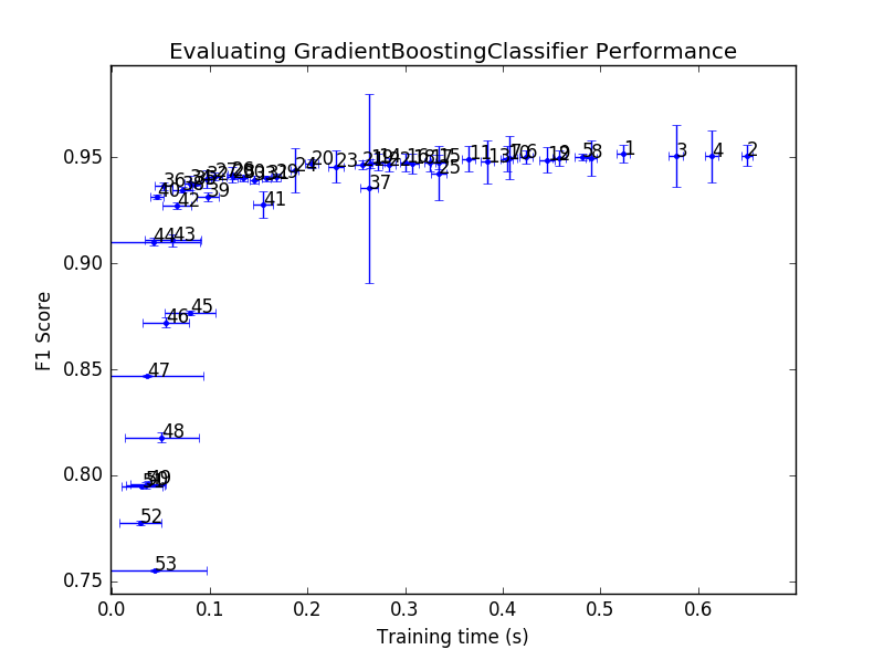
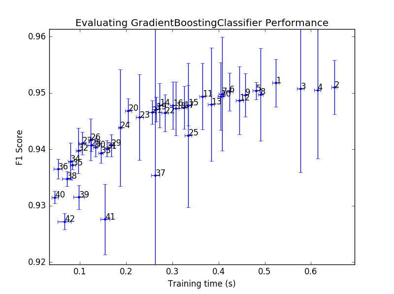
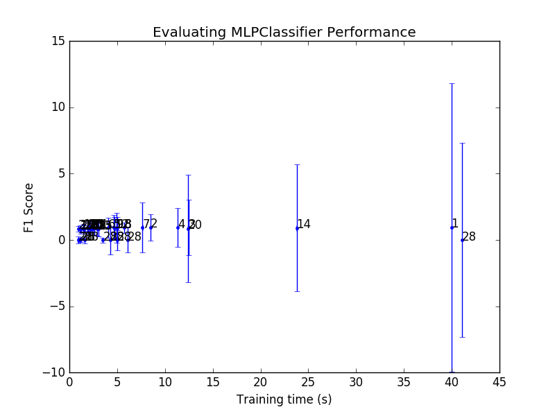
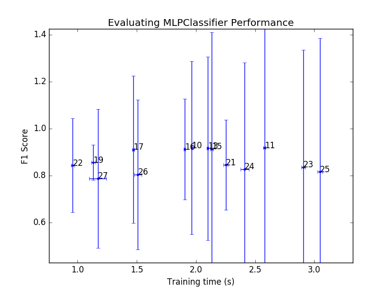
uncertainty for each of these scores.

# Train the inputted classifier using a stratified K-fold approach
# (split into 5) and evaluates the performance using cross validation
# Inputs:
#   - clf is the classifier defined from scikit-learn
#   - arrInput is a numpy array of shape n_samples, n_features
#   - arrTarget is a numpy array of shape n_samples
#   - show_report is a boolean value on whether to print the report to screen
# Returns:
#   - dict with trained_clf and the performance values

import numpy as np
from sklearn.model_selection import StratifiedKFold
from sklearn.metrics import accuracy_score, f1_score, precision_score, recall_score

def train_classifier(clf, arrInput, arrTarget, show_report=False):

	# Generate K-fold splitting
	skf = StratifiedKFold(n_splits=5, shuffle=True)

	# Initialise performance metrics
	accuracy = []
	precision = []
	recall = []
	F1 = []

	# Train the classifier for each K-fold split
	for train_index, test_index in skf.split(arrInput, arrTarget):
		X_train, X_test = arrInput[train_index], arrInput[test_index]
		y_train, y_test = arrTarget[train_index], arrTarget[test_index]

		# Train the classifier on the train data
		clf.fit(X_train, y_train)

		# Generate the cross val predictions on the test data
		y_pred = clf.predict(X_test)

		# Calculate performance metrics
		accuracy.append(accuracy_score(y_test, y_pred))
		precision.append(precision_score(y_test, y_pred))
		recall.append(recall_score(y_test, y_pred))
		F1.append(f1_score(y_test, y_pred))

	# Compute the combined mean and 2 sigma error for the K-fold iterations
	accuracy = [np.mean(accuracy), 2*np.std(accuracy)]
	precision = [np.mean(precision), 2*np.std(precision)]
	recall = [np.mean(recall), 2*np.std(recall)]
	F1 = [np.mean(F1), 2*np.std(F1)]

	# Print the performance metrics of the classifier (opt)
	if show_report == True:
		print("**** Training Report from KFold cross validation ****")
		print("Accuracy: {:.4f} +/- {:.4f}.".format(accuracy[0], accuracy[1]) )
		print("Precision: {:.4f} +/- {:.4f}.".format(precision[0], precision[1]) )
		print("Recall: {:.4f} +/- {:.4f}.".format(recall[0], recall[1]) )
		print("F1 score: {:.4f} +/- {:.4f}.".format(F1[0], F1[1]) )
		print("")

	return {'trained_clf': clf,
			'accuracy': accuracy,
			'precision': precision,
			'recall': recall,
			'F1': F1}

The data needs to be split into a training and testing sets and also scaled as some of the algorithms are scale invariant. The test_train_split and StandardScaler methods are well suited for performing these tasks. I split the data 80:20 training versus testing and StandardScaler will normalise the mean of the data to 0 and +/-1 as a standard deviation.

The classifiers I want to test are:

  • Logistic regression: plain old linear regression with a sigmoid activation function on the output layer. This is the most simple classifier and I find it to be a good indicator that the data preprocessing is working as intended. If the data has any complexity at all, this classifier should fail.
  • Support vector machines: with linear, polynomial and RBF kernels. These classifiers are able to draw more complex decision boundaries than a logistic regression algorithm. They can be slow to train.
  • Nearest K-neighbours: using 5 neighbours. This classifier optimises decision boundaries based on maximising the distance between the nearest neighbours of different classes.
  • Neural networks: with 1, 2, and 3 hidden layers. Neural networks have one of the biggest sets of hyperparameters to optimise for. I have found that using up to the square root of the number of features of hidden layers generally gives an idea of whether the neural network algorithm will be suitable. In this analysis I have chosen 3 network architectures with 1 hidden layer of 100 neurons, 2 hidden layers of 100 and 50 neurons, and 3 hidden layers of 100, 50 and 25 neurons.
  • Ensemble methods: Random forest, AdaBoost, and GBRT. These methods sort of perform their own feature formation. Random forest generates several decision trees based on dominant subsets of the features and then the output of each tree is averaged to form the final classification. AdaBoost and GBRT are boosting techniques that optimise several models that only perform better than average and are then combined together to “boost” the overall performance of the classifier.
# My analysis methods
import hr
# Import the classifiers to use from scikit-learn
from sklearn.linear_model import LogisticRegression
from sklearn.svm import SVC
from sklearn.neighbors import KNeighborsClassifier
from sklearn.neural_network import MLPClassifier
from sklearn.ensemble import RandomForestClassifier, AdaBoostClassifier, GradientBoostingClassifier
# Extra utilites from scikit-learn
from sklearn.preprocessing import StandardScaler
from sklearn.model_selection import train_test_split
from sklearn.metrics import classification_report

# Load in the HR data
(arrInput, arrTarget) = hr.load_hr_data()
# Split data into training and testing sets
TrainInput, TestInput, TrainTarget, TestTarget = train_test_split(
	arrInput, arrTarget, test_size=0.2)
# Use standard scaler to scale features -1 to +1 mean and std
scaler = StandardScaler()
ScaledTrainInput = scaler.fit_transform(TrainInput)
ScaledTestInput = scaler.transform(TestInput)

# Define the classifiers to train on the data
classifier_algorithms = {
    'Logistic Regression': LogisticRegression(),
    'Linear SVM': SVC(kernel='linear'),
    'Poly SVM': SVC(kernel='poly'),
    'RBF SVM': SVC(kernel='rbf'),
    'K Neighbours': KNeighborsClassifier(),
    '1 Layer NN (100)': MLPClassifier(),
    '2 Layer NN (100,50)': MLPClassifier(hidden_layer_sizes=(100,50)),
    '3 Layer NN (100,50,25)': MLPClassifier(hidden_layer_sizes=(100,50,25)),
    'Ada Boost': AdaBoostClassifier(),
    'Gradient Boosting': GradientBoostingClassifier(),
    'Random Forest': RandomForestClassifier()
}

# Train the algorithms on the data
trained_networks = list()
for clf_name, clf in classifier_algorithms.items():
	# Train the classifier and return the network and the scores in a dict
	training_output = hr.train_classifier(clf, ScaledTrainInput, TrainTarget)
	# Add the network name into the returned dict and append to trained_networks
	training_output.update({'Network Type': clf_name})
	trained_networks.append(training_output)
	#Evaluate the classifier performance and print the classification report
	Predictions = training_output['trained_clf'].predict(ScaledTestInput)
	print("Using the {} classifier:".format(clf_name))
        print("Accuracy: {:.2f}".format((TestTarget == Predictions).sum()/len(Predictions)) )
	print(classification_report(TestTarget, Predictions))
	print("")

The results show that the 3 best machine learning algorithms to use on this dataset (in order from best to worst) are: random forest, GBRT, and a 2-layer neural network. The random forest algorithm was able to achieve an accuracy of 99% and a precision of 1.00. Therefore the algorithm correctly identified all of the employees that were predicted as leavers but misidentified some employees as stayers when they were leavers. In this scenario, recall should be preferred over precision as it is more important to identify all of the leavers with a small collateral of misidentified stayers than it is to misidentify some of the leavers as stayers. I’ll leave precision-recall curve analysis for the next blog post.

Network Type Accuracy Precision Recall F1 Score
Logistic regression 79% 0.61 0.35 0.44
Linear SVM 78% 0.62 0.25 0.36
Polynomial SVM 95% 0.91 0.89 0.90
RBF SVM 96% 0.93 0.89 0.91
K neighbours 95% 0.89 0.91 0.90
1-layer neural network 97% 0.95 0.90 0.93
2-layer neural network 97% 0.96 0.92 0.94
3-layer neural network 97% 0.95 0.92 0.93
AdaBoost 96% 0.93 0.91 0.92
Gradient boosting 97% 0.97 0.91 0.94
Random forest 99% 1.00 0.94 0.97

The other 2 algorithms had slightly reduced accuracy, precision and recall scores. These algorithms are still quite encouraging as the scores are all above 0.9 using only the default parameters that are specified by scikit-learn. In my next blog post, I will take the top 3 performing algorithms and do some tweaking in the extended parameter space to see what algorithm can outperform the others in terms of accuracy metrics and training time.

First blog post

Hello World.

I  am currently working on up-skilling into the field of Data Science from an experimental physics reasearch background. There is a lot of overlap between the two fields: in physics a model is developed by considering the fundamental forces of nature and then this is tested by measuring some data and seeing how the two compare. In data science, the modelling process is not wholly thought up and performed by people, rather, machine learning is used in this step. Both of these fields require a human to oversee the modelling process to ensure that statistically significant predictions can be generated. This is the step that I enjoy the most: processing and analysing data and modelling techniques to ensure high quality predictions can be made.

In this blog, I will post a few of the personal projects I have been working on in my spare time. Some will be succesful and others may not be because sometimes we learn more from constant failure than instant success.

I am currently working on a stock analysis neural network code (based on the python scikit-learn package) and hope to have a post up about it soon. I’m calling it ShareBrained.