This post is continuing the analysis of the HR dataset from kaggle.com. In my last blog post, I looked at a broad range of learning algorithms from scikit-learn to see what fit the dataset best. In doing this I only used the default settings for each of the algorithms (except the neural networks where I defined the hidden layers). Now I will investigate the top 3 algorithms further by tuning the hyperparameters away from the default settings. I hope to find out which algorithm will outperform the others in terms of F1 score and training time.
Methodology
The way in which I will optimise the various algorithm’s hyperparamters is to use scikit-learn’s inbuilt grid search. This allows me to enter in the parameters I would like to check over and then it will train the algorithm using all of the possible combinations. Each hyperparameter grid search is performed 5 times using a stratified K-fold cross validation set so some simple statistics can be taken to test the reliability and robustness.
def optimise_classifier_f1(clf, parameter_grid, arrInput, arrTarget):
    # Generate cross validation set
    cv_splits = StratifiedKFold(n_splits=5, shuffle=True)

    # Perform grid search over paramter grid
    grid_search = GridSearchCV(
        estimator=clf,
        param_grid=parameter_grid,
        cv=cv_splits,
        scoring='f1'
        )
    grid_search.fit(arrInput, arrTarget)

    # Performance metrics from grid search
    fit_time = grid_search.cv_results_['mean_fit_time']
    fit_time_err = grid_search.cv_results_['std_fit_time']
    test_score = grid_search.cv_results_['mean_test_score']
    test_score_err = grid_search.cv_results_['std_test_score']
    rank_test_score = grid_search.cv_results_['rank_test_score']
    params = grid_search.cv_results_['params']

    # Print each point's rank and parameters
    print()
    print("Rank and parameters for: {}".format(type(clf).__name__))
    for i,j in zip(rank_test_score,params):
        print("Rank {0:2d}  Parameters {1:}".format(i,j))

    # Plot the performance graph with each point's rank
    fig, ax = plt.subplots(1,1)
    ax.errorbar(fit_time, test_score, fit_time_err, test_score_err, 'b.')
    ax.set_xlabel('Training time (s)')
    ax.set_ylabel('F1 Score')
    ax.set_title('Evaluating {} Performance'.format(type(clf).__name__))
    for x,y,rank in zip(fit_time, test_score, rank_test_score):
        ax.annotate(rank, xy=(x,y), textcoords='data')
    plt.show()
To visualise the performance of each classifier in the hyperparamter grid search, I have chosen to plot the F1 score versus the training time. F1 score is a good indicator of combined precision/recall score and the training time looks at the complexity of the model as a more complex algorithm will take longer to train. In this manner I can also compare the training time of different algorithms. Errorbars are plotted on both axes as that is a good way to distinguish if an algorithm can be reliably trained with the hyperparameters. The plot also contains the rank that each data point came in the overall grid search. Python prints out the rank and parameters of each datapoint to the terminal so I can see what was used.
Evaluating the gradient boosting algorithm
From the initial analysis of the gradient boosting algorithm, the default settings from scikit-learn gave a F1 score of 0.94. The two hyperparameters that I will concentrate my efforts on are the number of estimators and the maximum numbers of features.
# Optimise the gradient boosting classifier
clf = GradientBoostingClassifier()
parameter_grid = {
    'n_estimators':[10, 20, 40, 80, 120, 160],
    'max_features':[i for i in range(1,10)]
}
hr.optimise_classifier_f1(clf, parameter_grid, ScaledTrainInput, TrainTarget)
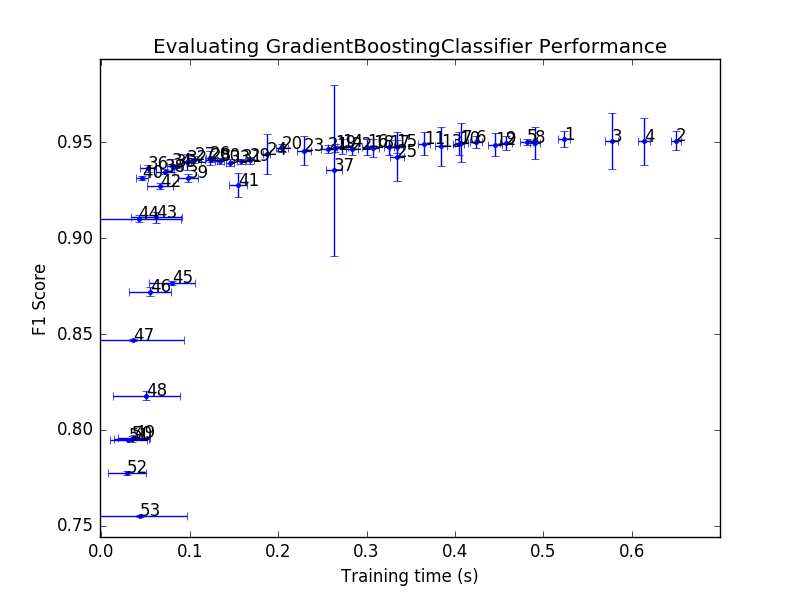
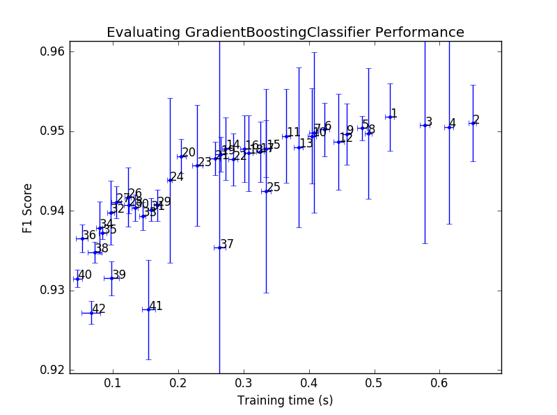
The above two figures are the results for the hyperparameter grid search, with the second figure just being a zoomed in version of the top figure. From these, it is apparent that the F1 score of 0.94 that was given with the default settings can’t really be improved on by a lot as the best performance is just above 0.95. The highest ranking F1 score (denoted by rank 1) was trained using hyperparameters of max_features=6 and n_indicators=160. I would suggest that the optimal hyperparameters for this algorithm is located at rank 20 with max_features=3 and n_indicators=80. The rank 20 datapoint has a small F1 errorbar which implies that it was reliably trained on each cross validation set. The training time errorbar is similar to all other datapoints around it, suggesting that gradient boosting isn’t having difficulty finding a solution. By chosing the rank 20 hyperparameters over the rank 1, the training time is reduced by a factor of 2.5 while the F1 score only decreases by less than 5%. In fact the errorbars of rank 1 and rank 20 overlap which implies that sometimes both algorithms train to the same F1 score.
Evaluating the 2-layered neural network
In the initial analysis of a 2-layered neural network on the dataset I used 100 and 50 neurons in each hidden layer. This gave an F1 score of 0.94, similar in performance to the gradient boosting algorithm. For the neural network I will concentrate on the regularisation parameter, alpha, and the number of neurons in each hidden layer.
# Optimise the 2-layer neural network
clf = MLPClassifier()
parameter_grid = {
    'hidden_layer_sizes':[(i,j) for i in [5,50,500] for j in [5,50,500]],
    'alpha':[0.0001, 1, 10, 1000]
}
hr.optimise_classifier_f1(clf, parameter_grid, ScaledTrainInput, TrainTarget)
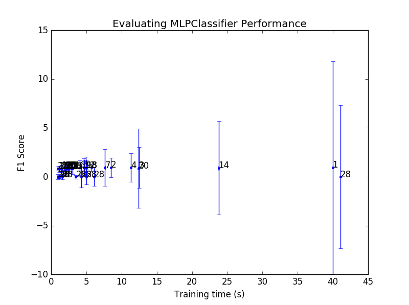
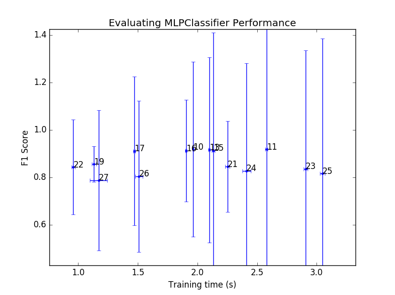
The results from the hyperparameter grid search on the 2-layer neural network is quite surprising in that the errorbars for the F1 score are all very large. The large error in these ponts indicates that the algorithm couldn’t be trained reliably. For each of the 5 cross validation sets there was a large range of F1 scores attained. It should also be noted that the training times are much larger than those for the gradient boosting algorithm. The 2-layered neural network algorithm can be ruled out for further investigation as it gives much worse performance. This also demonstrates why this type of analysis is important as the first impression given by the default settings of this algorithm had a performance that was in the top 3 of all tested.
Evaluating the random forest algorithm
The final algorithm to evaluate and find the optimal hyperparameters for is the random forest. This algorithm had the highest performance of all those initially evaluated with a F1 score of 0.97. The hyperparameters worth investigating are the number of estimators and the maximum number of features that the algorithm can utilise.
# Optimise the random forest classifier
clf = RandomForestClassifier()
parameter_grid = {
    'n_estimators':[i for i in range(1,20,2)],
    'max_features':[2,4,6]
}
hr.optimise_classifier_f1(clf, parameter_grid, ScaledTrainInput, TrainTarget)
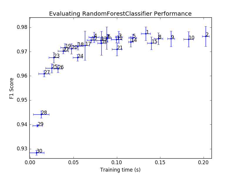
The performance curve for this classifier algorithm cements its position as being superior to the others. All but 1 datapoint have a higher F1 score than the highest datapoint in the gradient boosting algorithm. The errorbars are also quite stable between datapoints to indicate that this algorithm can be reliably trained on the dataset each and every time. The rank 1 datapoint used n_estimators=17 and max_features=4. I would choose the rank 4 datapoint as being optimal for this algorithm due to it taking half the time to train and still having a F1 score that overlaps with the rank 1 point. The hyperparameters for the rank 4 point are n_estimators=13 and max_features=2.
Overall
The final conclusion of this evaluation is that the random forest classifier algorithm is superior in F1 score and training time when compared to the other competing algorithms. Using a gradient boosting algorithm is the next best although training times are increased by a factor of 4 and the F1 score is 5% worse over the optimal. The 2-layered neural network was the worst performing with large training times and a high degree of variability in the F1 score of the trained networks.
In a future blog post I will finish this analysis by looking at the precision and recall scores as well as the confusion matrix for the random forest classifier using the optimal hyperparameters.
